Matrix Product Operator

Thomas E. Baker—August 18, 2015

Using the matrix product state (MPS) is a good starting point to find the ground state of at least 1D gapped Hamiltonians, though it may be useful elsewhere. Since the MPS rewrites the wavefunction in terms of a site by site decomposition, we need to look for a site by site decomposition of the Hamiltonian so it can connect with the MPS.

In this article, we will describe the connection between MPOs and operators, how they are written diagrammatically, and how this works for a 2D system. Details of how to write MPOs in ITensor automatically with AutoMPO and manually are located in the links.

Examples

The matrix product operator (MPO) can represent any operator in quantum mechanics that we'd like it to. The general rule for MPOs is that it is a matrix containing operators that only act on one site. An example of an MPO for the Hamiltonian of an Ising spin chain is

where @@I@@ is an identity matrix. When multiplied by other MPOs in the chain, we will accumulate terms in the lower left corner until we develop the full Hamiltonian.

When multiplied out fully, the MPO should return the full Hamiltonian. Not all sites need to have square MPOs. They can be of any size (and in general, the MPO is not unique!). At the first and last sites, the MPO looks like

Multiplying this out gives the full Hamiltonian

The ITensor code uses AutoMPO with the code

SpinHalf sites(N);
auto J=1;
AutoMPO ampo(sites);
for(int j = 1; j <= N; ++j)
{
ampo += J,"Sz",j,"Sz",j+1;
}
auto H = MPO(ampo);

Let's take a look at an MPO for a Heisenberg model:

with boundary MPOs

These MPOs multiply to the correct Hamiltonian:

The ITensor code is

SpinHalf sites(N);
auto J=1;
AutoMPO ampo(sites);
for(int j = 1; j <= N; ++j)
{
ampo += (J/2),"S+",j,"S-",j+1;
ampo += (J/2),"S-",j,"S+",j+1;
ampo += J,"Sz",j,"Sz",j+1;
}
auto H = MPO(ampo);

MPO Diagrams and Operators

A diagram for an MPO may look like

In ITensor, one of the vertical lines has a different prime level than the bottom leg. Both vertical legs have the same Index name, however.

SpinHalf sites;
ITensor H = MPO(sites);

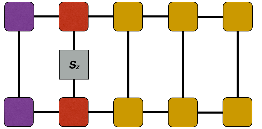
Note that each Hamiltonian has many diagrams added together. Our examples of the Ising and Heisenberg Hamiltonians above contain the sum of many diagrams which is why we choose to represent them as grey boxes.

To get access to the operators, one may fix the sub-indices on an MPO (i.e., @@a_1@@ and @@a_2@@ in @@\mathcal{H}_{a_1a_2}^{\sigma_2\sigma_3}@@ ). Fixing the indices to be 3 and 2 in the Ising model gives the @@S^z@@ operator. We can insert this operator only into the network to measure the onsite magnetization

psi.position(2);
auto C = dag(prime(psi.A(2),Site)) * sites.op("Sz",2) * psi.A(2);

That is how operators connect with MPOs and can be used in computation. They are defined in the SiteSet if another operator, other than Sz is needed.

2D Systems

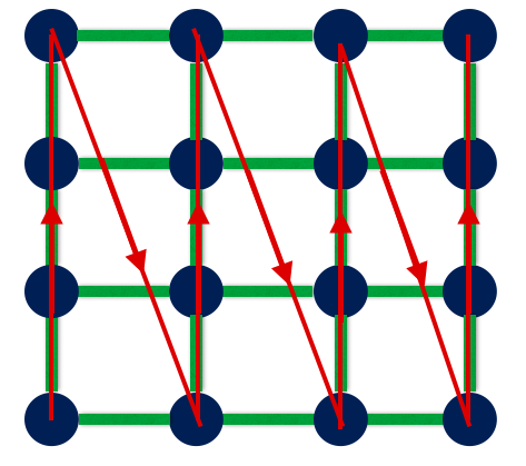
2D systems can be mapped onto a 1D system. Consider a square lattice:

The red lines show how we want to move over the lattice as we solve it, for example, with a DMRG calculation. Note that unlike our 1D chains with near-neighbor bonds, there are horizontal bonds (green bars). Sometimes the path is drawn differently in papers, but this is the path taken.

The cost of mapping the 2D calculation to a 1D problem is the introduction of bonds that are not just near-neighbor terms. The associated network would look like

The complications of this diagram can be summarized by examining the bulk MPO (some middle site) for a 4x4 Heisenberg model as shown above as

auto Nx = 4;//Number of sites in the x-direction
auto Ny = 4;//Number of sites in the y-direction
auto N = Nx * Ny;
auto J = 1;
SpinHalf sites(N);
auto lattice = heisenberg(Nx,Ny);
AutoMPO ampo(sites);
for(auto b: lattice)
{
ampo += (J/2),"S+",b.i1,"S-",b.i2;
ampo += (J/2),"S-",b.i1,"S+",b.i2;
ampo +=     J,"Sz",b.i1,"Sz",b.i2;
}
auto H = MPO(ampo);
dmrg(psi,H,sweeps);

This matrix is much larger and shows that increasing the range of the entanglement is driving the sizes of our MPOs larger and larger. DMRG is known to be a minimally entangled method that works best with short range interactions. Writing MPOs that connect farther and farther points make the entanglement entropy larger over a longer area, but the fundamental point is that the matrix sizes increase. So, practically, the computational steps slow down.

We should also mention that one could write down an MPO for a DMRG algorithm that goes from site 1 to site 8 to site 3 to site 12 to site 6 to site 5, etc. But writing the MPO that connects adjacent sites is best for fast computation.

Periodic Boundary Conditions

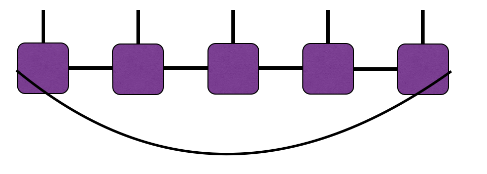
We can now see why the periodic boundary conditions affect the computational speed of a calculation. The difference between the open boundary condition and the periodic boundary condition for the Ising model is a term @@S_1^zS_N^z@@ .

But our matrix on each site can no longer be the comparatively small @@3 x 3@@ matrix that makes computation fast. We need the operator on site 1 to connect all the way to site @@N@@ . We won't bother writing out the MPO that does this, but we will just reinforce that increasing matrix size increases computational time.

The ITensor code is very small, however, to produce this large matrix.

SpinHalf sites(N);
auto J=1;
AutoMPO ampo(sites);
for(int j = 1; j <= N; ++j)
{
ampo += J,"Sz",j,"Sz",j+1;
}
ampo += J,"Sz",1,"Sz",N;
auto H = MPO(ampo);

Exponential Interactions

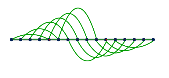
The summary statement is that long range entanglement causes a method like DMRG to go much slower due to the increased MPO size, but this is not a strict statement. Some long range terms can be encoded into small MPOs. Since MPOs are not unique, finding small representations for different operators is crucial. For example, an exponential function has the simple form

where @@\lambda=\exp(-1)@@ . Multiplying this out gives the full exponential and makes distant sites interact. This also avoids a situation where long range entanglement occurs by writing out each equivalent interaction in a larger matrix. The exponential is naturally encoded in the MPO for its small size.