Estimating the Cost of and Efficiently Contracting a Tensor Network

Thomas E. Baker—August 17, 2015

Your computer only has a certain number of operations it can perform per second. Making a program that uses the least amount of steps to get the answer means that less of your computer time is used. More calculations can be done. And wouldn't your advisor like that (and you might too)!

The difference between providing an algorithm that scales like @@m^4@@ operations and @@m^{12}@@ operations could mean that one can study a larger system in a shorter amount of time. Some systems might not be accessible at all with the @@m^{12}@@ scaling relation. This could be the difference between a few minutes of calculation time versus many hours or even days.

In this article, we will discuss how to estimate the cost of contracting a tensor network and the best algorithm for doing so. We also demonstrate how to measure a correlation function with the least number of operations.

Cost of Contractions

Each line represents a variable in a sum. For the case of a typical tensor occurring in a matrix product state, the legs often have different numbers of terms that must be summed.

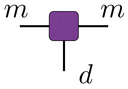
The horizontal lines contain @@m@@ terms (although in general, the left and right legs do not need to have the same number of terms). This number is called the bond dimension and can be thought of as the size of the wavefunction on each site in an MPS (meaning, the size of the local MPS matrix for that site). Specifically for DMRG, this number corresponds to the number of many body states kept in the Schmidt decomposition.

The vertical leg corresponds to the physical index, @@d@@ , and typically ranges over only a few values. The bond dimension may range over thousands of values.

Note that if we carry out the sum of the following diagram on the bond marked with a pale green box, we would perform @@m^3@@ operations to perform the sum on that single bond.

Highlighting the bond in green means we are interested in summing over the index corresponding to that bond. We can think of the cost of summing @@\mu@@ as being propotional too the number of terms involving a @@\mu@@ in them. Counting these terms up, we see that there are two tensors and they have three unique indices between them. To evaluate the sum, we need to perform @@m\times m\times m=m^3@@ operations (for performing operations on @@\sigma@@ , @@\mu@@ , and @@\nu@@ ). We can also find this number quickly and visually by counting the number of legs touching the tensors that a chosen line touches.

For another example,

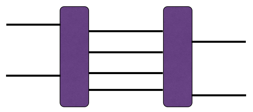
is of order @@\mathcal{O}(m^8)@@ since the internal lines touch two tensors and these touch eight lines collectively. To see this explicitly, consider one of the lines in between the two tensors (one that touches both blocks). Each of the blocks is connected to 7 other lines. In total, that is eight lines and if each line (corresponding to an index) has @@m@@ components, then the cost is of @@m^8@@ . This is not to say that each line requires this cost to contract, but to evaluate the whole network, we need to pay attention to the largest cost of all the pairwise sums.

For a chain of @@L@@ tensors (we discuss specifically tensors in an MPS here) the cost of calculation is @@\mathcal{O}(Ldm^3)@@ . When reporting the cost of a computation, we often do not report the @@L@@ variable since this is considered fixed in the computational cost. We can only change the exponent of @@m@@ with any algorithm we choose.

Contraction Example @@\mathcal{O}(dm^4)@@

Let's take a look first at an inefficient way to calculate the contracted tensor network. It works; it gives the right answer, but it's not the best we can do.

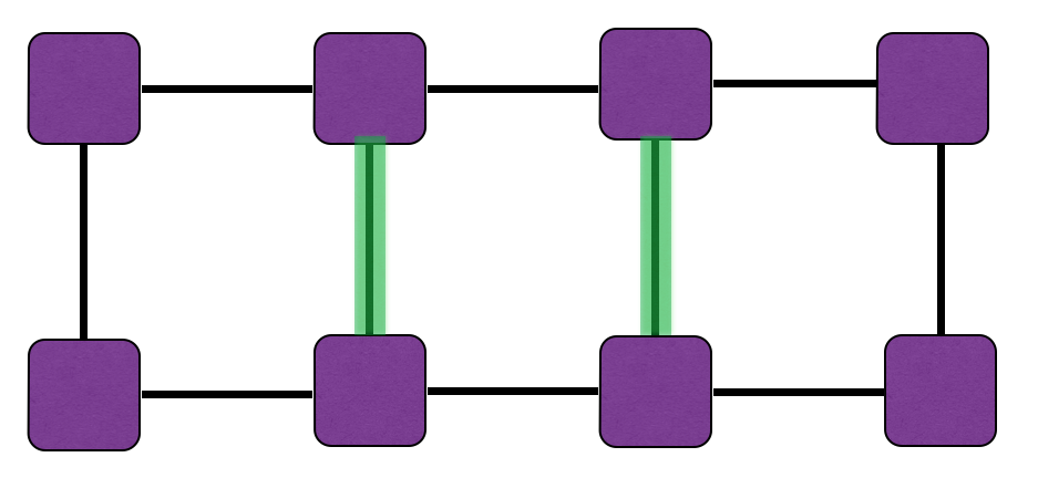
The cost to evaluate this is @@\mathcal{O}(dm^4)@@ . So, starting from one of the bonds on the inside of the chain is not as efficient as we can make the algorithm.

The most efficient algorithm @@\mathcal{O}(dm^3)@@

This algorithm is used in correlation functions in ITensor. We'll skip a detailed discussion of how to implement this algorithm here and just report the cost at each step.

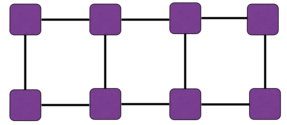
The bonds touching the green bond (below) have two indices of size @@m@@ while the bond itself has @@d@@ . So the cost of evaluating only this bond is @@\mathcal{O}(dm^2)@@ .

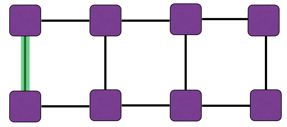
Contracting these bonds leaves us with a choice. We choose to contract the top horizontal bond next:

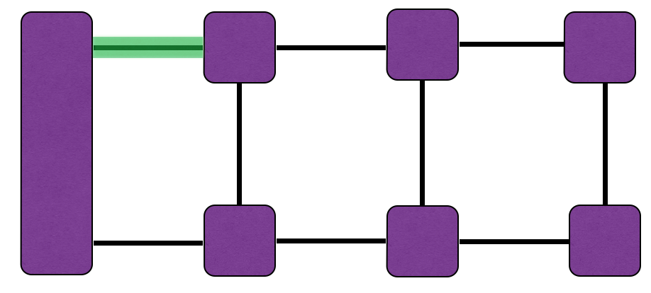
The size of the index relating to the green box is now @@m@@ . Examining the large, rectangular tensor on the left, it touches the green bond and one other bond of size @@m@@ . The other tensor that the green bond touches connects to an index of size @@d@@ and another index of size @@m@@ . The cost is @@\mathcal{O}(dm^3)@@ . This is larger than our first step and is the important number to keep in mind. If we find a cost higher than this, than that would be the cost (but we won't).

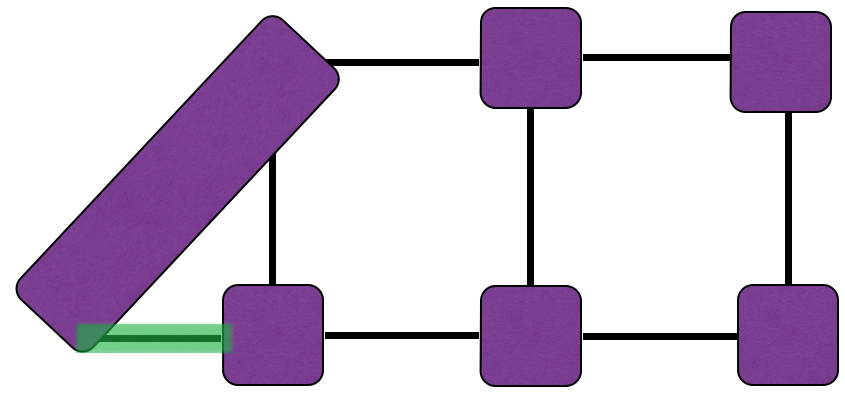
The next bond to contract has an equal cost:

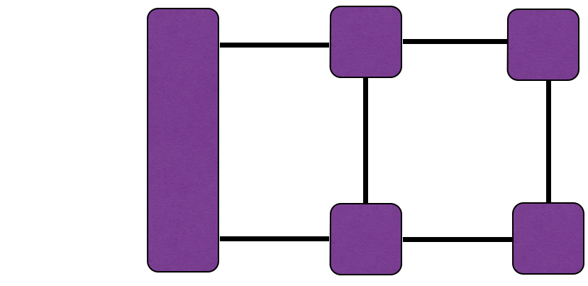
We have obtained a diagram we had two steps ago. The process repeats for as many tensors as we have in the network. But we now know the cost.